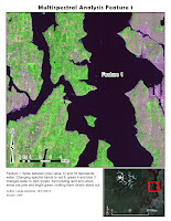
 This map shows the shallow waters along the coast to the West of the gap, located at x: 470000 and y: 3355000. The water West of the gap is much warmer, as shown by the yellowish striations. The water on the East side of the gap is much deeper, as shown by the blue color, lacking the warmth represented by yellow. The actual striation in the warm, shallow water are caused by waves and tidal action that is more pronounced in the shallow waters.
I found this feature as I was looking along the coast and I noticed that the seas side of the coastline showed a lot of temperature variation between the coastal water on the east and west side of the gap. After examining aerial photos, there did not seem to be any correlation between water temperature and urban development along the coast.
Using the band combination of Red 2, Green 1 and Blue 6, the warm, shallow water displayed in yellow. In contrast vegetation and most of urban areas display in blue, and cool , deep water pourple-blue.
 In Lab 7 we learned to locate and identify surface features based on their pixel value. Using tools provided by ERDAS Imagine Histogram tool I found the specific peaks in pixel values. Then using the Inquire Cursor I located areas on the image that matched those pixel values.
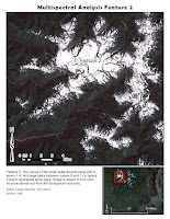
Then I identified those areas, and adjusted color bands to bring out areas of interest from their background. In the case of the second map, the snow capped mountain peak, no adjustment from true color was needed. This is because white snow cap clearly stands out from the mountain and vegetation color. Third image is that of shallow water with heavy sediment load. The challenge was to bring out the sediment pattern in the water. Under most band variations the sediment pattern was very difficult or impossible to distinguish from deep water. However using red 4, green 2 and blue 1, the eddies in the water popped out very clearly.
In this lab we used ArcMap and ERDAS Imagine to modify remote sensing data. This is done through application of various filters. The two programs used, ArcMap and ERDAS, provide certain benefits and work best when are used in tandem to overcome the limitations associated with each one.
In Module 5 we learned to calculate the relationship between wavelength and frequency, and to calculate the energy based on the wavelength. The basic principle is that the shorter the wavelength the greater the energy of the particle.
Then we were introduced to ERDAS IMAGINE software, and learned some of its basic utilities, including how to save your work without the software crashing.
Last part of the exercise was to use ERDAS software to select an area of a larger project area, calculate land area of each feature in it, and export it. Calculating land area involved editing the attribute table and adding another column. Then we imported the file into ArcMap, and created a usable map out of it.
In lab 4 we did ground truthing. This involves checking and comparing the land use that we determined in Lab 3 to the actual land usage. This is done in a number of ways, but with the limitation we had (such as this being an online course) we used Google Maps. For most features in the mapped area street view was sufficient to determine the actual land usage. Some areas not adjacent to the road required zooming in really close and using associated features to determine actual land usage.
The points that were ground truthed were chosen randomly, though there are other, more methodical ways to select points for ground truthing.
This week's assignment was to identify general land use and land cover types from an aerial photo. I used the skills learned from Lab 2, and identify land features mostly based on tone and, more importantly, texture. Combined with recognizing features by size and association, I could narrow down and label trailer park, grocery stores, and small commercial buildings.
Module 2 lab focused on basics of visual interpretation of aerial photos. In the first exercise we identified different tones, or shades, of surface features. We also identified varying ground textures. These varied from very fine, smooth water surface, all the way to very coarse thick forest. Once the tones and textures were identified we had to outline them using ArcMap.
 In the second exercise we had to identify surface features on an aerial photo based on shape and size, pattern, shadow, and association. Size and shape was useful for recognizing houses, cars, and roads. Shadow was useful for tall features, such as trees and a water tower. Pattern was very useful for identifying waves on the water, parking stripes in the parking lot, and a neighborhood with houses along a street. Last was association. A swimming pool, black rectangle of water in a neighborhood, and a pier, thin, long structure jutting out into the water. As in the first exercise, we used ArcMap to mark and label the features.
 This map shows the shallow waters along the coast to the West of the gap, located at x: 470000 and y: 3355000. The water West of the gap is much warmer, as shown by the yellowish striations. The water on the East side of the gap is much deeper, as shown by the blue color, lacking the warmth represented by yellow. The actual striation in the warm, shallow water are caused by waves and tidal action that is more pronounced in the shallow waters.


