GIS 4043 Final

   The final project for GIS 4043 is an analysis of a preferred corridor for Bobwhite-Manatee Transmission Line Project. Analysis included determining number of houses within the corridor and within a 400 foot buffer around the corridor. Number of schools and day-cares in the same area. This was dine by looking at areal images of the area and digitizing all the buildings within those two zones.
   Further, I used ArcMap to determine the acreage of  environmentally sensitive areas in the corridor. Those areas included swamps, streams, bayous, as well as environmental conservation areas. This was done by intersecting wetlands layer with the corridor, and clipping conservation areas to the corridor. In both cases the new layers we added to the Final geodatabase file I created for this project.
    As for the base map, instead of using aerials as a base, I used a basic map. I chose this because the presentation was supposed to be for a wide audience, and this background would make it clear where this are is supposed to be.

Here is the PowerPoint presentation.

Here is the slide by slide presentation.

Module 13: Final

The final project for GIS 3015 is a map, created for The Washington Post, which shows ACT data for the year 2013 by using skills and techniques learned throughout the semester. As part of this assignment, we were to find the applicable data, convert it into a format usable by ArcMap, download the correct shapefile and project it to a usable projection. Once the data was obtained, the map could be created with those data sets using the Gestalt principles learned during the course. The final map represents two data sets: the average ACT score for each state and the percentage of graduating students that took the ACT per state. Both data sets were created in Excel and joined with the Attribute Table of the base map. Then the data was classified, using the Natural Breaks classification. Map insets were used to show states outside the lower 48. Also an inset map of the Northeast to show data for all the small states that would otherwise be covered by the thematic symbols.

Week 13 - Georeferencing, Editing and ArcScene

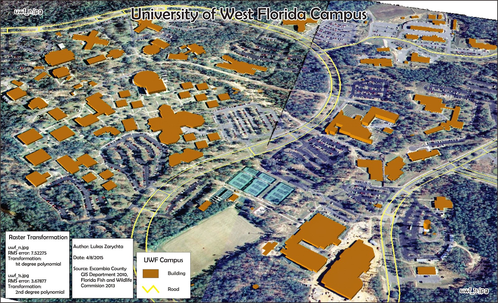 The last (but not final) assignment for the class focused on georeferencing an image, editing features and using ArcScene. First part of the assignment was to take an aerial image of an area and georeference it. That is, to assign it a spatial properties, give it a place in the world. That is done using the Georeference toolbar by connecting a point on the unreferenced image to a point with a known location. You should have at least 10 locations connected that way, and those locations should be spread out throughout the image. Avoid choosing locations that is in a line, or that are clustered closely together.

Second part consisted of editing features. In this case adding a building and a road based on previously referenced image. Other than steps needed to start, save and end editing, this works a lot like most drawing programs. Once drawn, data was added to the attribute table in order to use it later on in ArcScene. Last part of creating this map included adding an eagle nest, creating a double buffer around it, and linking a web address of it's picture.

Third part of the assignment involved using ArcScene to create a 3d image of UWF campus. Using Extrude tool all buildings were given appropriate heights. This is were adding building height to the newly created building in the attribute table came in.

Module 12: NeoCartography/ Google Earth

In this module we used one of the previously created maps and convert it to a file format compatible with Google Earth. The image included here shows a map of South Florida from Module 10, displayed on Google Earth. That part of assignment involved taking a map in ArcGIS, converting it into KMZ file, and opening it in Google Earth. Second part of the assignment involved repeating the above process, but with only a single layer (South Florida counties in my case). Third and final part of the assignment involved making a video tour of high population areas in South Florida, zooming in/out and rotating the camera to show the 3d buildings, and doing all of it with tool provided only by Google Earth.

Week 12 - Network Analysis/Geocoding & Model Builder

Map on the lest shows EMS stations in Lake County, Florida. This was the first part of the assignment, geocoding, which is assigning street addresses to location on the map. This is done with the use of geocoding tools, though some location may not be assigned an address automatically. In those cases we used Google Earth to locate the EMS stations, and then picked the correct address from the list of possible ones.

The second part of the assignment involved Network Analysis and creating a route. This is shown in the inset map. Using Network Analysis tool is somewhat involved, as it uses data based on specific data and time to calculate the route. 

Module 11: 3D Mapping

In Module 11 we learned about 3D mapping. This included using mainly ArcScence, but also ArcGlobe to a small extent. Exercises included creating basic 3D map, with graduated elevation colors, river layer, and points points of interest. Other exercises focused on using exaggeration tool to show elevation patterns in otherwise relatively flat area. Also using lighting to show elevation patterns, extruding features from 2D shapes, and extruding feature to an extent based on certain value (such a property value).

Finally we learned to create out of a 2D shapefile a 3D building footprint with actual building heights. Then we imported that 3D model into Google Earth, and displayed it on the Google Earth globe, in it's actual location.