Biscayne Shipwrecks: Analysis

 In this module we build up on the previous module to analyze the data. Using Buffers around the known shipwrecks, we found the types of sea floor types related to those ship wrecks. This way we can determine the types of environments that are conducive to ships wrecking.

Biscayne Shipwrecks - Prepare Week

In this module we are using methods utilized in previous modules to analyze seafloor of Biscayne Bay in search of shipwrecks. Data used for this is somewhat different than for terrestrial analysis. We are using bathymetric data, as well as navigational charts, both current and historical. Navigational charts, especially historic ones must be georeferenced, which may be difficult to get vary close due to erosion and fluctuating coastline.

Scythian Landscapes - Report

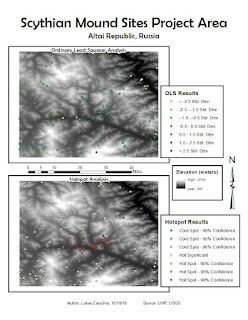
Data presented in this file shows spatial distribution of known Scythian burial mounds. Data also shows random points in the project area, and the probability of those points being a burial mound site. Secondary surfaces generated for analysis were slope, aspect, and elevation. Slope favored incline of less than 16%, aspect favored south facing slopes, and elevation favored areas below 2000 meters. Linear regression method used was Ordinary Least Squares analysis. Missing data includes mound site distance from the river. Limitation of this model the limited number of points used for spatial distribution of data.

                The OLS results include the adjusted R-squared value of 0.697804, which means the variables are explaining about 68% of site presence or absence. The coefficients are not near zero, and are mostly positive, which means they have a positive, direct influence on the data. The Spatial Autocorrelation test has the following z-score and p-value values: z-score of 13.834296 and p-value of 0.00000. The combination of high z-score and low p-value indicates a normal distribution of the data and spatially autocorrelated data.

Scythian Landscapes - Analyze Week

In this part of the module we prepared base data for Landscape Modeling of the region. From the raster created last week we created, we created a number of separate data rasters. 

Using last week's raster I extrapolated elevation values for the area. I used those values to determine slope steepness, and slope facing. In this case South facing slopes were more favorable to slopes facing other directions. I also created a contour map of the region.

Lastly, I created a shapefile with locations of Scythian burial mounds.

Scythian Landscapes - Prepare Week

First part of Scythian Landscapes module focused on preparing the data. This involved finding and downloading DEMs of the area, and creating a raster mosaic out of them. Then the mosaic raster was clopped to the provided study area shapefile.

Second part of the module was to take an aerial image of the mound site, and georeference it based on coordinates provided. Visual georeferencing was not possible, due to very poor resolution of the background image.

Predictive Modeling

In this module we performed predictive modelling of an area. The model was divided into three site categories, high, medium and low probability. These categories were based on slope and proximity to a waterway.

First I created a raster out of a mosaic of smaller rasters. Then I extrapolated elevation values for the area. I those values to determine slope steepness, and slope facing. In this case South facing slopes were more favorable to slopes facing other directions. Lastly I used a separate shapefile of streams and rivers in the area, created a buffer around it representing optimal settlement distance from the waterway. Lastly I combined the slope and waterway data to determine site probability in the area.

Finding Pyramids

During week 3 we identified possible pyramid locations in densely forested areas. The map included here shows area surrounding Angkor Wat it Cambodia. 

The supervised classification is based on false color infrared base raster image. Considering the base color band combination, any possible pyramid sites will be very difficult to spot, if not impossible. This is in part due to healthy vegetation overgrowing the ruins showing in the same shades and tones as all other healthy vegetation.

NDVI False Color measures greenness of the vegetation. It measures the difference between the Red and Near Infrared bands.

Lyr 451 depicts healthy vegetation in shades of reds, browns, oranges and yellows. Opened, developed areas appear in shades of white and near white colors. Adding mid infrared band allows for detection of stages of plant growth or stress.

Supervised Classification allows us to assign certain pixel values to specific objects. In turn, ArcMap extrapolates those values to the entire image.

Module 01 - Finding Maya Pyramids: Interpreting Remote Sensing Imagery for Archaeology

In module one we learned to use different combinations of color bands to create aerial images emphasizing various aspects of the image.
The top image is false color infrared, combining red, green, and near infrared bands. It is useful for identifying types and health of vegetation.
Middle image is true color, composed of blue, green, and red bands. It makes identifying certain features easier, since they appear on the image the same way they appear in real life.
The bottom image, Landsat 8, while it provides only shades of gray, it has the highest resolution of the three images.

Module 10 - Final Research Project

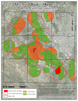
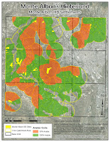My final project examines increase of catchment area of a community through creation of satellite communities. I examined Monte Alban IIIA and IIIB periods in the area directly around Monte Alban itself.

To get the data I needed, surface area statistics, I georeferenced and digitized the soil maps, then created separate shapefile with only the arable areas. Next I digitized the sites and created 1 Km buffer around them to represent the catchment area. The important part of this step was to "dissolve all" buffer zones, in order to create a single large area, rather than a number of overlapping circles. Then I clipped the soil map to the catchment area, create Thiessen polygons to divide the catchment area between all sites, and calculated surface areas for various types of soils.

Module 09 - Remote Sensing

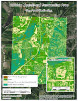
 In module 9 we classified data gathered with remote sensing techniques in two ways: unsupervised and supervised.

In unsupervised classification, we let the software classify pixels into a number of predetermined classes. The downside of this type of classification is that number of categories can overlap. Also some vastly different features may be assigned into the same category, because the shade and tone of their pixels is identical, or nearly so. In case of my unsupervised classification, ArcMap combined water and smooth surfaces such as roof tops into one category.

In supervised classification, we determine a number of points on the raster image, and assign each point a predetermined category (grass, trees, pavement, etc.). We then let the software process all the pixels, and assign them into the predetermined categories. This is still not without issues, as my buildings category and pavement/bare ground categories got combined, but there was a lot less redundant classification.

Module 08- 3D Modeling

In module 8 we created a 3d image of subsurface soil horizons. This process involved interpolating depth data from the shovel test information to create raster files representing elevation of each soil horizon. Then, using ArcScene, we displayed those rasters in a 3d image. To make the image easier to read, we increased the vertical scale, this created a comfortable distance between layers.

When looking at the shovel test data, we split it into three separate layers, one for each horizon, and assigned each horizon a different color. In both Fig 2 and 3 yellow represents A horizon, green B horizon, and purple C horizon.

Figure 4 is missing A horizon because there was no data associated with the given shapefile. While surface data may be available, it would most likely be inaccurate, because the initial data was not gathered from a site datum point, but from the surface. And depending on the region, surface can quickly change for many reasons, such as weather, land usage, etc.

Fig 2. Shovel Test data, divided into soil horizons.

Fig 1. Project area boundaries, horizontal and vertical.

Fig 3. Proposed subsurface line in the project area.

Fig 4. Soil horizons: B on top, C on the bottom.

Module 7- Surface Interpolation

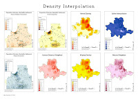
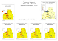
In the first part of module 7 we learned to import text and AutoCAD data into ArcMap. This usually involved converting the data into a correct table format, adding appropriate column headings, and assigning projection, if known.

In the second part of the module we learned to interpolate surface data based on known data points. This information can in turn be used to get an idea what the site looked like during the time period we are studying, or to narrow down good places for further studies of the site.

Module 06- Digitizing

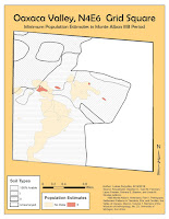In module 6 we learned to digitize old maps, and linking data tables to the shapefile's attribute table. 

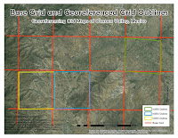First step in digitizing old maps is to georeference them, which was covered in module 5. The challenge in this exercise was in aligning independent site grids to a separate map showing the grid distribution. The problem was the poor quality of the grid distribution map, and parts of the grid were not visible and I had to interpolate the the full grid. In addition a lot of site grids were difficult to read, as a lot of notes on the maps were difficult to read, either due to poor hand writing or poor scan quality.

The second part of the exercise was to join a data table to the shapefile's attribute table. The challenge here is to create a data table from the old maps and reports that you are digitizing.

Module 05 - Georeferencing

In module 5 we learned to georeference images, historic maps in this case. Georeferencing means taking an image such as a historic map, aerial photo, etc., overlaying it on top of an already georeferenced map and adjusting it to correspond with georeferenced points.

Once you acquired a historic map or aerial photo, you need to import it into ArcMap. Also set up a background map to use as a reference. It may be helpful to import an additional background map, either street map or a topo map. This can make georeferencing easier. Then using Georeference Tool, link points on your image to the georeference background. The more linked points the better. These points may be topographical features such as island shores, hills, rivers. They may also be anthropological features: houses, roads, etc. You just need to keep in mind that a lot of these features may have changed over time.

Module 04 - Historic

In Module 4 we learned to find and incorporate historic data into maps. First part of the assignment was to find the historic data. While the historic map of Boston was provided by UWF, we used Ancestry.com to get census information about Paul Revere. 

Second part of the exercise focused on incorporating data into a map. This included creating internal and external links. External links hyperlink to Google Maps, the location in Boston with Paul Revere's house in. Internal links includes an image of a page from 1790 census, including entry for Paul Revere.

Module 03 - Ethics

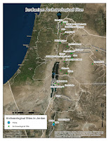In module 3 we covered the importance of ethics in archaeology. The reading points out that the need for codified ethics rules rose up from the wide spread of commercial archaeology. While I believe that is certainly not wrong, one cannot forget that until recently academia led archaeology was nothing more than glorified looting, to be shown off in the looter's national museums as a trophy. Any talk about ethics in archaeology cannot be focused on one aspect, such as CRM, but on all aspects. Academia is certainly not immune from people trying to profit from archaeological findings.

The lab for module 3 focused on creating shapefiles. This was done by either manually creating a point, and creating a shapefile out of it, or by importing a data table into ArcMap. The data table contained fields with site name, site description, and Lat and Long of the site. Once imported and converted into a shapefile, it displayed all the site in the database. When looking at the attached map, Petra site (in blue) is the manually created shapefile. All other sites come from a database that was converted into a shapefile.

Module 02 - Queries and Clips

In Module 02 we learned to perform SQL queries and to use the Clip tool of ArcMap. In this module we used these techniques to compare the areas and landmarks of Chicago before, and 20 years after the Great Chicago Fire.

The SQL query is a very useful tool for selecting a range of data from a larger database. The query is done by inserting an equation referencing file's attribute table into the tool. Once the query is run, the newly selected data can be exported into a separate shapefile. This provides a quick and relatively easy way to separate a large shapefile into a number of smaller ones that may offer more specific information. In the case of the Chicago Fire map, I have taken a shapefile with landmarks in Chicago, and created two separate file, one with all the landmarks build before the fire, and one with landmarks build between 1871 and 1890.

The Clip tool simply takes a shapefile, and removes all data from it that falls outside of another, related shapefile. In the case of the Chicago Fire map, once I had the pre 1871 landmark file, and 1871-1890 landmark file, I clipped to their respective city shapefiles. The pre 1871 landmarks file was clipped to the Chicago 1869 map, thus removing all landmarks outside the city limits. The 1871-1890 landmark file was clipped to the Chicago 1890 map, again removing all landmarks that fell outside the city limits at the time.