Scythian Landscapes - Prepare Week

First part of Scythian Landscapes module focused on preparing the data. This involved finding and downloading DEMs of the area, and creating a raster mosaic out of them. Then the mosaic raster was clopped to the provided study area shapefile.

Second part of the module was to take an aerial image of the mound site, and georeference it based on coordinates provided. Visual georeferencing was not possible, due to very poor resolution of the background image.

Predictive Modeling

In this module we performed predictive modelling of an area. The model was divided into three site categories, high, medium and low probability. These categories were based on slope and proximity to a waterway.

First I created a raster out of a mosaic of smaller rasters. Then I extrapolated elevation values for the area. I those values to determine slope steepness, and slope facing. In this case South facing slopes were more favorable to slopes facing other directions. Lastly I used a separate shapefile of streams and rivers in the area, created a buffer around it representing optimal settlement distance from the waterway. Lastly I combined the slope and waterway data to determine site probability in the area.

Finding Pyramids

During week 3 we identified possible pyramid locations in densely forested areas. The map included here shows area surrounding Angkor Wat it Cambodia. 

The supervised classification is based on false color infrared base raster image. Considering the base color band combination, any possible pyramid sites will be very difficult to spot, if not impossible. This is in part due to healthy vegetation overgrowing the ruins showing in the same shades and tones as all other healthy vegetation.

NDVI False Color measures greenness of the vegetation. It measures the difference between the Red and Near Infrared bands.

Lyr 451 depicts healthy vegetation in shades of reds, browns, oranges and yellows. Opened, developed areas appear in shades of white and near white colors. Adding mid infrared band allows for detection of stages of plant growth or stress.

Supervised Classification allows us to assign certain pixel values to specific objects. In turn, ArcMap extrapolates those values to the entire image.

Module 01 - Finding Maya Pyramids: Interpreting Remote Sensing Imagery for Archaeology

In module one we learned to use different combinations of color bands to create aerial images emphasizing various aspects of the image.
The top image is false color infrared, combining red, green, and near infrared bands. It is useful for identifying types and health of vegetation.
Middle image is true color, composed of blue, green, and red bands. It makes identifying certain features easier, since they appear on the image the same way they appear in real life.
The bottom image, Landsat 8, while it provides only shades of gray, it has the highest resolution of the three images.

Module 10 - Final Research Project

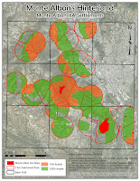
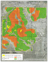My final project examines increase of catchment area of a community through creation of satellite communities. I examined Monte Alban IIIA and IIIB periods in the area directly around Monte Alban itself.

To get the data I needed, surface area statistics, I georeferenced and digitized the soil maps, then created separate shapefile with only the arable areas. Next I digitized the sites and created 1 Km buffer around them to represent the catchment area. The important part of this step was to "dissolve all" buffer zones, in order to create a single large area, rather than a number of overlapping circles. Then I clipped the soil map to the catchment area, create Thiessen polygons to divide the catchment area between all sites, and calculated surface areas for various types of soils.

Module 09 - Remote Sensing

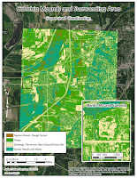 In module 9 we classified data gathered with remote sensing techniques in two ways: unsupervised and supervised.

In unsupervised classification, we let the software classify pixels into a number of predetermined classes. The downside of this type of classification is that number of categories can overlap. Also some vastly different features may be assigned into the same category, because the shade and tone of their pixels is identical, or nearly so. In case of my unsupervised classification, ArcMap combined water and smooth surfaces such as roof tops into one category.

In supervised classification, we determine a number of points on the raster image, and assign each point a predetermined category (grass, trees, pavement, etc.). We then let the software process all the pixels, and assign them into the predetermined categories. This is still not without issues, as my buildings category and pavement/bare ground categories got combined, but there was a lot less redundant classification.